3 Simple Ways to Rotate Charts in Excel

Whether you're managing data for a business report, a scientific study, or personal budgeting, rotating charts in Excel can greatly improve visual presentation, readability, and analysis. Excel offers several techniques to manipulate charts for more dynamic presentations. Here are three simple and effective methods to rotate your charts and achieve the perfect visual angle for your data.
Method 1: Using 3D Rotation Tool
Excel provides a built-in feature to rotate charts in three dimensions, allowing for depth, height, and angle adjustments. Here’s how you can use it:
- Select your chart: Click on the chart to activate it.
- Access Chart Tools: Go to the “Chart Tools” context tabs.
- Open 3-D Rotation: Navigate to the “Layout” tab, then find and click on “3-D Rotation.”
- Adjust Rotation: Here, you can change:
- X Rotation: Rotates the chart horizontally.
- Y Rotation: Rotates the chart vertically.
- Z Rotation: Rotates the perspective or depth of the chart.
⚠️ Note: Be cautious when rotating charts as excessive rotation can make data difficult to read or distort proportions.
Method 2: Using Excel Formulas
If you’re looking for a more precise rotation, Excel formulas can be employed to manipulate the angle of your charts:
- Create a Chart: First, generate your basic chart.
- Add Helper Columns: Use helper columns to calculate new coordinates for each point, adjusting their angle. You can use trigonometric functions like
SINandCOSto determine the new positions.
Original X Original Y Theta (Angle) New X New Y 2 3 45° =A2*COS(C2)-B2*SIN(C2) =A2*SIN(C2)+B2*COS(C2) - Plot New Coordinates: After calculating new positions, plot these to see the rotated chart.
Method 3: Copy and Paste Special
Although not a traditional rotation, this method allows you to simulate rotation through different formatting:
- Select the Chart: Click to activate it.
- Copy the Chart: Use Ctrl+C or right-click and select “Copy.”
- Paste Special: Go to a blank area of the spreadsheet, right-click, select “Paste Special,” then choose “Picture” or “Picture (Enhanced Metafile).”
- Rotate: Once pasted, you can rotate the image by dragging its corners or by using the “Format” tab for precise adjustments.
✅ Note: This method changes the chart to an image, making further data manipulation impossible. Use it for presentations or static documents.
Rotating charts in Excel offers flexibility in data presentation, enabling you to emphasize trends, compare datasets, or simply enhance aesthetic appeal. Whether through direct manipulation with the 3D rotation tool, using formulas for precise adjustments, or transforming the chart into a picture for rotation, Excel provides multiple approaches to achieve the desired visual outcome. Each method has its place depending on your needs, from real-time data analysis to static reporting. Remember, while rotation can make charts more visually appealing, it's crucial to ensure that your data remains clear and the integrity of your presentation is maintained.
How do I rotate charts to a specific angle in Excel?
+Use the 3-D Rotation tool under Chart Tools or manipulate the data with formulas to rotate charts to a specific angle.
Can I rotate charts using macros?
+Yes, VBA macros can be used to rotate charts programmatically in Excel.
Does rotating charts affect the data accuracy?
+Rotation does not alter the data itself, but excessive rotation can make interpretation challenging, especially for 3D charts.
Related Terms:
- How to rotate chart Excel
- excel rotate radar chart
- change chart direction in excel
- how to flip excel chart
- flip axis on excel chart
- excel chart reverse order


