Compare Excel Columns: Find Matches Easily

In the realm of data management, Excel is a powerful tool used by millions worldwide to organize, analyze, and manipulate data efficiently. One common task that many users find themselves doing is comparing columns to identify matches or differences between datasets. This process is essential in scenarios like reconciling financial records, merging customer databases, or detecting duplicates. In this extensive guide, we'll explore several methods to compare columns in Excel, ensuring you can find matches easily, regardless of the complexity of your data.
Why Compare Columns in Excel?
Before delving into the how-to, let's understand why column comparison is a pivotal operation:
- To find duplicate entries across lists or datasets.
- To verify data consistency, which is crucial for accurate reporting or analysis.
- To prepare data for merging, ensuring unique entries are preserved.
- To highlight discrepancies or errors in datasets, especially when reconciling data from different sources.
Method 1: Using Conditional Formatting
Conditional formatting is a simple yet effective way to highlight matches or differences between columns:
- Select the columns you want to compare. For example, click on the header of Column A and drag to the last cell of Column B.
- Go to the Home tab, find the Styles group, and click on Conditional Formatting.
- Choose New Rule, then select Use a formula to determine which cells to format.
- In the formula box, enter a formula like
=A1=B1(assuming your data starts at row 1). This formula will check if the values in Column A match those in Column B. - Click Format, choose a format (e.g., a different color for cells where the formula holds true), then confirm with OK.
- Excel will now highlight cells where the entries match, based on your chosen format.
💡 Note: Make sure your range selection includes both columns, or the formatting won't apply correctly. Also, the formula should compare cells in relative fashion, adjusting for your data's starting point.
Method 2: Utilizing VLOOKUP Function
The VLOOKUP function is a popular choice for finding matches between two columns, especially when you want to find matches from one column within another:
- In a new column adjacent to the one you want to check for matches, enter the VLOOKUP formula.
- The formula structure is:
=VLOOKUP(A2,$C$2:$D$100,2,FALSE), where:- A2 is the lookup value you're searching for.
- $C$2:$D$100 is the table array to search in (ensure it has no headers).
- 2 specifies which column to return the result from (here, the second column).
- FALSE ensures an exact match is returned, not an approximate one.
- If a match is found, VLOOKUP will return the value from the second column of the array; if not, it returns an error which you can handle with an IFERROR or manually.
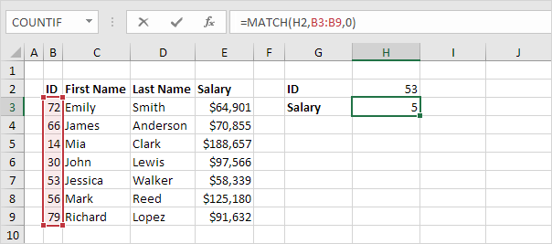
Method 3: Using Excel's MATCH Function
The MATCH function can help you identify where your matches occur within a column:
- In an empty column next to the column you want to compare, enter the formula
=MATCH(A2, $C$2:$C$100, 0), where:- A2 is the cell you're checking for a match.
- $C$2:$C$100 is the range to search within.
- 0 specifies an exact match.
- If there is a match, the formula will return the row number of the match within the specified range. If no match is found, it will return #N/A.
This method provides the exact position of matches, which can be particularly useful for further data manipulation or analysis.
Comparing Multiple Columns: A Practical Example
Suppose you have a sales dataset where you want to compare sales figures for three consecutive months. Here’s how you can do it:

| Month 1 | Month 2 | Month 3 | Formula | Result |
|---|---|---|---|---|
| 500 | 450 | 475 | =A2=B2=C2 | FALSE |
| 600 | 600 | 600 | =A3=B3=C3 | TRUE |
| 300 | 350 | 375 | =A4=B4=C4 | FALSE |
This approach helps in identifying trends, anomalies, or consistent figures across multiple columns for effective analysis.
Advanced: Using Power Query for Comparison
For more complex datasets or when dealing with large amounts of data, Power Query in Excel can be your ally:
- Select your data and go to the Data tab, then click on From Table/Range.
- In the Power Query Editor, use the Merge Queries feature to combine data from different tables or compare columns:
- Choose the table or range to compare with your current query.
- Specify how the data should be matched, often by selecting a common key column.
- Once merged, you can filter, sort, or transform the data as needed.
- Click Close & Load to return the result to Excel.
💡 Note: Power Query is particularly useful for comparing data across multiple worksheets or even different Excel files. It also allows for repeated, consistent data transformation processes.
Final Thoughts on Column Comparison
Comparing columns in Excel is a versatile task that can be approached through various methods depending on the complexity of your data, your familiarity with Excel functions, and the level of detail you require. Each method has its advantages:
- Conditional Formatting is great for visual quick checks.
- VLOOKUP and MATCH functions provide more detailed insights into where matches occur.
- Power Query offers advanced capabilities for comparing large datasets or when consistent data transformation is necessary.
Choosing the right technique depends on your dataset's size, the complexity of the comparison, and what subsequent actions you plan with the found matches. Remember, Excel's prowess lies in its flexibility, allowing you to tailor your comparison methods to your specific needs.
Can I compare more than two columns in Excel?
+Yes, you can compare multiple columns using various methods. VLOOKUP or MATCH functions can be expanded, or Power Query can handle complex comparisons across multiple columns.
What do I do if my columns contain text and not numbers?
+The methods work the same for text as they do for numbers. Ensure your comparison formulas compare the text accurately, case-sensitive if needed.
How do I handle errors in VLOOKUP or MATCH functions?
+Use the IFERROR function to handle errors gracefully. For example, =IFERROR(VLOOKUP(A2,C2:D100,2,FALSE),“Not Found”) will return “Not Found” if the VLOOKUP returns an error.
Related Terms:
- Compare data Excel
- Compare Excel online
- VLOOKUP compare two columns
- Compare 2 table in Excel
- Cara Compare data Excel
- Compare text Excel


