5 Easy Ways to Compare Lists in Excel

When working with large datasets in Microsoft Excel, it's common to need to compare lists or datasets to find matches, differences, or to manage inventory, databases, or any other data-heavy tasks. Here are five straightforward methods to compare lists in Excel that range from basic to advanced, ensuring you can work efficiently with your data.

Method 1: Using VLOOKUP

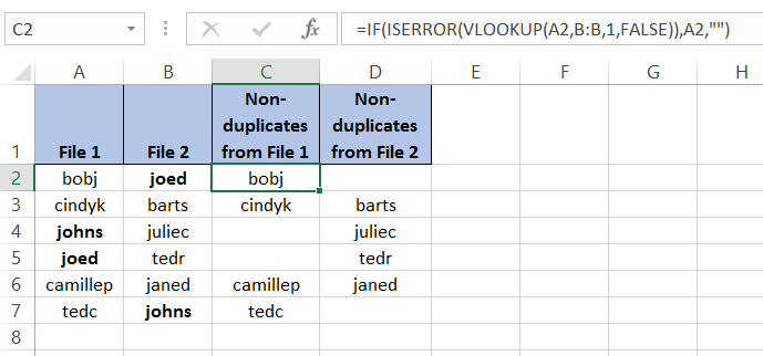
The VLOOKUP function is one of Excel’s most popular features for data comparison. Here’s how you can use it to compare two lists:

• Prepare your data: Ensure both lists have a common identifier, like an ID or name.
• Syntax: =VLOOKUP(lookup_value, table_array, col_index_num, [range_lookup])
• Usage:
  1. Enter VLOOKUP in the formula bar.
  2. The lookup_value is the value from the first list you want to check against the second list.
  3. The table_array is the range of the second list, starting from the column containing the lookup_value.
  4. Set col_index_num as the number of columns away from the lookup column to the column you want to retrieve.
  5. For an exact match, use FALSE for range_lookup.

📌 Note: VLOOKUP can be slow on large datasets; consider using INDEX and MATCH for larger lists for better performance.

Method 2: Conditional Formatting

If you’re looking to highlight differences or matches visually, conditional formatting is your go-to method:

• Select both lists.
• Navigate to “Home” > “Conditional Formatting”.
• Choose “New Rule” and then “Use a formula to determine which cells to format”.
• Enter a formula like =A1<>B1 or =A1=B1 depending on if you want to highlight mismatches or matches.
• Choose a formatting style.

Method 3: Pivot Tables

Pivot tables are excellent for summarizing data and comparing lists for summary statistics or to find duplicates:

• Insert a pivot table from your combined data set.
• Drag the columns you want to compare into the rows and values area.
• Use filters to drill down into data for detailed comparison.

Method 4: Advanced Filter

This method helps in extracting unique or duplicate records between lists:

• Go to “Data” > “Advanced” > “Filter”.
• Select the range of your first list and the criteria range from the second list.
• Choose the action you want, like finding unique records or duplicates.

Method 5: Using Power Query

For those who handle large datasets, Power Query offers powerful tools to merge, compare, and clean data:

• Open Power Query from the “Data” tab.
• Load both lists into Power Query.
• Use “Merge Queries” to join your lists based on common fields.
• Apply transformations like “Remove Duplicates” or “Group By” for detailed comparison.

📌 Note: Power Query requires Excel 2010 or later versions for access to these advanced features.

In summary, Excel offers a variety of tools to compare lists effectively. Whether you're looking for matches or differences, or managing large datasets, these methods provide the flexibility needed to get the job done. The choice between VLOOKUP, conditional formatting, pivot tables, advanced filter, or Power Query depends on the size of your lists, the complexity of your data, and your familiarity with Excel's features. Each method has its own strengths, allowing you to tailor your approach based on the specific needs of your project or task.

Related Terms:

• Compare 2 table in Excel
• Compare Excel online
• Compare two list
• excel formula to compare lists
• excel matching two lists
• cross reference two lists excel