How to Easily Compare Two Lists in Excel for Matches

In the world of data analysis, Microsoft Excel is a key tool used by professionals across various industries to manage, organize, and analyze data efficiently. One common task that users often find themselves performing is comparing two lists to find matches or differences. Whether you are reconciling financial records, merging mailing lists, or cleaning up databases, knowing how to compare lists in Excel can save you considerable time and reduce errors. In this detailed guide, we will explore several methods to compare two lists in Excel for matches.
Understanding the Basics of Comparing Lists in Excel
Before we dive into the different methods, let’s understand why we need to compare lists:
- Data Validation: Ensure data integrity by matching records from different sources.
- Data Merging: Combine data from multiple lists while avoiding duplicates.
- Change Tracking: Identify changes or updates in datasets over time.
Method 1: VLOOKUP Function
VLOOKUP, or Vertical Lookup, is one of the simplest functions for finding matches between two lists.
Steps to Use VLOOKUP:
- Place your first list in column A and the second list in column C. Use column B for the results.
- In cell B2, type:
=VLOOKUP(A2, C2:C1000, 1, FALSE), assuming your second list ends at row 1000. Here:- A2 is the lookup value.
- C2:C1000 is the lookup range.
- 1 means to return the value from the first column of the lookup range.
- FALSE ensures an exact match.
- Drag the formula down to fill the rest of column B.
🔍 Note: VLOOKUP will return “#N/A” if no match is found, helping you identify non-matching entries.
Method 2: Conditional Formatting
Conditional formatting visually highlights matching or unique values:
Steps to Apply Conditional Formatting:
- Select the range you want to format (e.g., your first list).
- Go to Home > Conditional Formatting > New Rule.
- Choose “Use a formula to determine which cells to format.”
- Enter a formula like
=COUNTIF(C2:C1000, A2)>0assuming your second list is in column C. - Choose a format (e.g., fill color) to highlight the matches.
- Click OK to apply the rule.
This method is particularly useful for quick visual analysis.
Method 3: Using Excel Tables and Filters
Excel’s Table feature with filters can streamline the comparison process:
Steps to Use Tables and Filters:
- Select your lists and convert them into tables by pressing Ctrl + T.
- Activate filters on each table by selecting them and going to Home > Sort & Filter > Filter.
- Sort or filter one list to show only unique values, or use Advanced Filter to display only the matching or unique values across the lists.
Method 4: Using Power Query
Power Query, part of Excel’s Get & Transform tools, can automate the comparison of large datasets:
Steps to Use Power Query:
- Go to Data > Get Data > From Table/Range to load both lists into Power Query.
- Use the Merge Queries feature to join these lists based on the columns you want to compare.
- Specify how you want to match (Full Outer, Left Outer, etc.) to find matches or mismatches.
- Load the result back into Excel for further analysis.
Advanced Techniques
If basic methods don’t suffice, consider:
- Array Formulas: Use complex formulas like
=IF(ISERROR(MATCH(A2, C2:C1000, 0)),“No Match”,“Match”)to compare lists. - Matching with Additional Conditions: Use INDEX and MATCH functions or more complex VLOOKUP for conditional matches.
🚀 Note: Advanced techniques require a better understanding of Excel functions and might be overkill for simple comparisons but are invaluable for large or complex data sets.
Comparing lists in Excel for matches is not just about finding similarities or differences but also about leveraging Excel's powerful tools to ensure data accuracy and integrity. Whether you're a beginner using basic functions like VLOOKUP or a seasoned analyst utilizing Power Query for large datasets, Excel offers a range of solutions to make list comparison an easy task.
What if my lists are in different worksheets or workbooks?
+You can use the same VLOOKUP function by specifying the workbook and sheet name in the range. For instance, =VLOOKUP(A2, [WorkbookName]SheetName!C2:C1000, 1, FALSE).
How can I find items in List A that are not in List B?
+Use the ISNA function with MATCH or VLOOKUP. For example: =IF(ISNA(MATCH(A2, C2:C1000, 0)),“Not in List B”,“In List B”).
Is there a way to compare lists with slight variations in text?
+Yes, use the EXACT function for case-sensitive comparison, or you might need to clean and standardize the data first before comparison.
Can I automate this process with Excel Macros or VBA?
+Absolutely, using VBA, you can automate list comparison, which can be particularly useful if you have to perform this task frequently.
Related Terms:
- VLOOKUP to compare two lists
- find matches in two lists
- excel compare 2 list


