Chi Square Test in Excel: A Step-by-Step Guide
The Chi-Square test is a statistical method used to determine if there is a significant difference between the expected frequencies and the observed frequencies in one or more categories. It is often used in hypothesis testing to check whether two variables are related or if distributions of a categorical variable differ from one another. This guide will walk you through how to perform a Chi-Square test in Microsoft Excel, breaking down each step for clarity.
Understanding the Chi-Square Test

Before diving into the practical steps in Excel, let's grasp the basic concept:
- Data Requirements: You need categorical (discrete) data.
- Null Hypothesis: Assumes no difference or association between categories.
- Chi-Square Statistic: Measures how much observed counts deviate from the expected counts under the null hypothesis.
Preparation
To conduct a Chi-Square test in Excel, you'll need:
- A data set with categorical variables.
- Basic understanding of Excel functions and formulas.
Step-by-Step Guide
Collecting Data
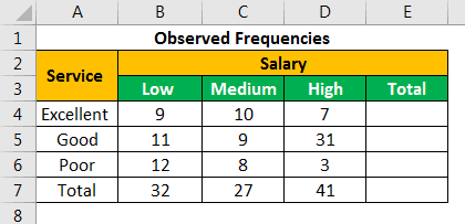
Start by gathering your data. Here’s a hypothetical example:
| Category A | Category B | |
|---|---|---|
| Group X | 30 | 20 |
| Group Y | 45 | 55 |
Calculate Expected Frequencies
The expected frequencies (E) for each cell can be calculated as:
- E = (Row Total * Column Total) / Grand Total
Here’s how to compute this in Excel:
=((C4+C5)*(B3+C3))/(B4+C4+B5+C5)
📝 Note: Ensure your data layout is consistent with the example above for easy reference in formulas.
Chi-Square Calculation
Now, calculate the Chi-Square statistic using this formula:
- χ² = Σ [(O - E)² / E], where O is the observed frequency, and E is the expected frequency.
Here’s the Excel formula for each cell:
=((B4-((C4+C5)(B3+C3)/(B4+C4+B5+C5)))^2)/(((C4+C5)(B3+C3)/(B4+C4+B5+C5)))
Sum these values for the total Chi-Square statistic.
Critical Value and P-Value
Excel’s CHISQ.DIST.RT function can help determine the P-value:
=CHISQ.DIST.RT(chi-square statistic, degrees of freedom)
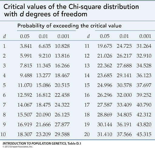
And compare this with the critical value from a Chi-Square distribution table or use Excel’s CHISQ.INV.RT function to find the critical value at a given significance level.
Interpreting Results
Compare your calculated Chi-Square value with the critical value or consider the P-value:
- If P-value ≤ α (commonly 0.05), reject the null hypothesis.
- If P-value > α, do not reject the null hypothesis.
In summary, using the Chi-Square test in Excel allows you to assess whether observed frequencies differ significantly from expected frequencies, offering insights into categorical data relationships or distribution comparisons. By following these steps, you’ve harnessed Excel’s capabilities to perform statistical analysis efficiently. Remember, while Excel simplifies calculations, the interpretation of results requires a good understanding of statistics. Thus, always check your understanding and seek guidance if needed.
What is the difference between Chi-Square test and a t-test?
+
The Chi-Square test is used for categorical data to determine if there’s a significant difference between observed and expected frequencies. A t-test, on the other hand, is used for continuous data to compare means between two groups.
Can I use Chi-Square test for continuous data?
+
No, the Chi-Square test is not appropriate for continuous data. You would need to categorize the continuous data into bins or use other tests like ANOVA or t-tests, which are designed for continuous data.
How do I determine the degrees of freedom in a Chi-Square test?
+
The degrees of freedom for a Chi-Square test is calculated as (number of rows - 1) * (number of columns - 1).
Related Terms:
- chi square formula copy paste
- chi square calculator excel
- calculate test statistic in excel
- chi square test statistic formula
- how to calculate chi square
- chi square critical value excel
